Piping in Python - Data Analysis with Python

Abstract¶

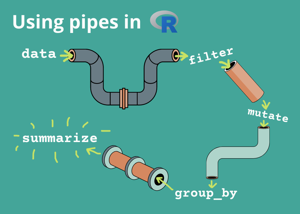
Piping is a programming paradigm that allows chaining multiple operations together in a readable and concise manner. It is inspired by the pipe operator (%>%) in R’s dplyr package and is implemented in Python using libraries like dfply. This approach is particularly useful for data manipulation tasks, as it enables a clean and logical flow of operations on data.

Keywords:datastatisticsdata analysispython¶

Piping in Python¶

Learn how to summarize the columns available in an R data frame. You will also learn how to chain operations together with the pipe operator, and how to compute grouped summaries using.

The dfply package makes it possible to do R’s dplyr-style data manipulation with pipes in python on pandas DataFrames.

dfply website here

Key Features of Piping:

Chaining Operations: Use the >> operator to chain multiple operations on a pandas DataFrame.
Deferred Evaluation: Operations are recorded symbolically and evaluated only when needed.
Readable Syntax: Makes complex data transformations easier to read and understand.

Common Functions in dfply:

select(): Select specific columns.
drop(): Drop specific columns.
filter(): Filter rows based on conditions.
mutate(): Add or modify columns.
summarize(): Compute summary statistics.
group_by(): Group data for aggregation.

Piping simplifies workflows by reducing the need for intermediate variables and making the code more intuitive

import pandas as pd
import seaborn as sns
cars = sns.load_dataset('mpg')
from dfply import *
cars >> head(3)

The >> and >>=¶

dfply works directly on pandas DataFrames, chaining operations on the data with the >> operator, or alternatively starting with >>= for inplace operations.

The X DataFrame symbol

The DataFrame as it is passed through the piping operations is represented by the symbol X. It records the actions you want to take (represented by the Intention class), but does not evaluate them until the appropriate time. Operations on the DataFrame are deferred. Selecting two of the columns, for example, can be done using the symbolic X DataFrame during the piping operations.

Exercise 1.¶

Select the columns ‘mpg’ and ‘horsepower’ from the cars DataFrame.

# your solution goes here

Selecting and dropping¶

There are two functions for selection, inverse of each other: select and drop. The select and drop functions accept string labels, integer positions, and/or symbolically represented column names (X.column). They also accept symbolic “selection filter” functions, which will be covered shortly.

Exercise 2.¶

Select the columns ‘mpg’ and ‘horsepower’ from the cars DataFrame using the drop function.

# your solution goes here

Selection using ~¶

One particularly nice thing about dplyr’s selection functions is that you can drop columns inside of a select statement by putting a subtraction sign in front, like so: ... %>% select(-col). The same can be done in dfply, but instead of the subtraction operator you use the tilde ~.

Exercise 3.¶

Select all columns except ‘model_year’, and ‘name’ from the cars DataFrame.

# your solution goes here

Filtering columns¶

The vanilla select and drop functions are useful, but there are a variety of selection functions inspired by dplyr available to make selecting and dropping columns a breeze. These functions are intended to be put inside of the select and drop functions, and can be paired with the ~ inverter.

First, a quick rundown of the available functions:

starts_with(prefix): find columns that start with a string prefix.
ends_with(suffix): find columns that end with a string suffix.
contains(substr): find columns that contain a substring in their name.
everything(): all columns.
columns_between(start_col, end_col, inclusive=True): find columns between a specified start and end column. The inclusive boolean keyword argument indicates whether the end column should be included or not.
columns_to(end_col, inclusive=True): get columns up to a specified end column. The inclusive argument indicates whether the ending column should be included or not.
columns_from(start_col): get the columns starting at a specified column.

Exercise 4.¶

The selection filter functions are best explained by example. Let’s say I wanted to select only the columns that started with a “c”:

# your solution goes here

Exercise 5.¶

Select the columns that contain the substring “e” from the cars DataFrame.

# your solution goes here

Exercise 6.¶

Select the columns that are between ‘mpg’ and ‘origin’ from the cars DataFrame.

# your solution goes here

Subsetting and filtering¶

row_slice()¶

Slices of rows can be selected with the row_slice() function. You can pass single integer indices or a list of indices to select rows as with. This is going to be the same as using pandas’ .iloc.

Exercise 7.¶

Select the first three rows from the cars DataFrame.

# your solution goes here

distinct()¶

Selection of unique rows is done with distinct(), which similarly passes arguments and keyword arguments through to the DataFrame’s .drop_duplicates() method.

Exercise 8.¶

Select the unique rows from the ‘origin’ column in the cars DataFrame.

# your solution goes here

mask()¶

Filtering rows with logical criteria is done with mask(), which accepts boolean arrays “masking out” False labeled rows and keeping True labeled rows. These are best created with logical statements on symbolic Series objects as shown below. Multiple criteria can be supplied as arguments and their intersection will be used as the mask.

Exercise 9.¶

Filter the cars DataFrame to only include rows where the ‘mpg’ is greater than 20, origin Japan, and display the first three rows:

# your solution goes here

pull()¶

The pull() function is used to extract a single column from a DataFrame as a pandas Series. This is useful for passing a single column to a function or for further manipulation.

Exercise 10.¶

Extract the ‘mpg’ column from the cars DataFrame, japanese origin, model year 70s, and display the first three rows.

# your solution goes here

DataFrame transformation¶

mutate()

The mutate() function is used to create new columns or modify existing columns. It accepts keyword arguments of the form new_column_name = new_column_value, where new_column_value is a symbolic Series object.

Exercise 11.¶

Create a new column ‘mpg_per_cylinder’ in the cars DataFrame that is the result of dividing the ‘mpg’ column by the ‘cylinders’ column.

# your solution goes here

transmute()

The transmute() function is a combination of a mutate and a selection of the created variables.

Exercise 12.¶

Create a new column ‘mpg_per_cylinder’ in the cars DataFrame that is the result of dividing the ‘mpg’ column by the ‘cylinders’ column, and display only the new column.

# your solution goes here

Grouping¶

group_by() and ungroup()

The group_by() function is used to group the DataFrame by one or more columns. This is useful for creating groups of rows that can be summarized or transformed together. The ungroup() function is used to remove the grouping.

Exercise 13.¶

Group the cars DataFrame by the ‘origin’ column and calculate the lead of the ‘mpg’ column.

# your solution goes here

Reshaping¶

arrange()

The arrange() function is used to sort the DataFrame by one or more columns. This is useful for reordering the rows of the DataFrame.

Exercise 14.¶

Sort the cars DataFrame by the ‘mpg’ column in descending order.

# your solution goes here

rename()

The rename() function is used to rename columns in the DataFrame. It accepts keyword arguments of the form new_column_name = old_column_name.

Exercise 15.¶

Rename the ‘mpg’ column to ‘miles_per_gallon’ in the cars DataFrame.

# your solution goes here

gather()

The gather() function is used to reshape the DataFrame from wide to long format. It accepts keyword arguments of the form new_column_name = new_column_value, where new_column_value is a symbolic Series object.

Exercise 16.¶

Reshape the cars DataFrame from wide to long format by gathering the columns ‘mpg’, ‘horsepower’, ‘weight’, ‘acceleration’, and ‘displacement’ into a new column ‘variable’ and their values into a new column ‘value’.

# your solution goes here

spread()

Likewise, you can transform a “long” DataFrame into a “wide” format with the spread(key, values) function. Converting the previously created elongated DataFrame for example would be done like so.

Exercise 17.¶

Reshape the cars DataFrame from long to wide format by spreading the ‘variable’ column into columns and their values into the ‘value’ column.

# your solution goes here

Summarization¶

summarize()

The summarize() function is used to calculate summary statistics for groups of rows. It accepts keyword arguments of the form new_column_name = new_column_value, where new_column_value is a symbolic Series object.

Exercise 18.¶

Calculate the mean ‘mpg’ for each group of ‘origin’ in the cars DataFrame.

# your solution goes here

summarize_each()

The summarize_each() function is used to calculate summary statistics for groups of rows. It accepts keyword arguments of the form new_column_name = new_column_value, where new_column_value is a symbolic Series object.

Exercise 19.¶

Calculate the mean ‘mpg’ and ‘horsepower’ for each group of ‘origin’ in the cars DataFrame.

# your solution goes here

summarize() can of course be used with groupings as well.

Exercise 20.¶

Calculate the mean ‘mpg’ for each group of ‘origin’ and ‘model_year’ in the cars DataFrame.

# your solution goes here

Data Analysis with Python

Python Fundamentals 2.

Data Analysis with Python

Git and Version Control