Multivariate Statistics - Descriptive Statistics with Python

Abstract¶

This notebook explores multivariate relationships through linear regression analysis, highlighting its strengths and limitations. Practical examples and visualizations are provided to help users understand and apply these statistical concepts effectively.

Keywords:datastatisticsdata analysispython¶

Goals of this lecture¶

There are many ways to describe a distribution.

Here we will discuss:

Measurement of the relationship between distributions using linear, regression analysis.

Importing relevant libraries¶

import numpy as np
import matplotlib.pyplot as plt
import seaborn as sns ### importing seaborn
import pandas as pd
import scipy.stats as ss

%matplotlib inline 
%config InlineBackend.figure_format = 'retina'

import pandas as pd
df_estate = pd.read_csv("data/models/real_estate.csv")
df_estate.head(5)

Describing multivariate data with regression models¶

So far, we’ve been focusing on univariate and bivariate data: analysis.
What if we want to describe how two or more than two distributions relate to each other?

Let’s simplify variables’ names:

df_estate = df_estate.rename(columns={
    'house age': 'house_age_years',
    'house price of unit area': 'price_twd_msq',
    'number of convenience stores': 'n_convenience',
    'distance to the nearest MRT station': 'dist_to_mrt_m'
})

df_estate.head(5)

We can also perform binning for “house_age_years”:

df_estate['house_age_cat'] = pd.cut(
    df_estate['house_age_years'],
    bins=[0, 15, 30, 45],
    include_lowest=True,
    right=False
)
df_estate.head(5)

cat_dict = {
    pd.Interval(left=0, right=15, closed='left'): '0-15',
    pd.Interval(left=15, right=30, closed='left'): '15-30',
    pd.Interval(left=30, right=45, closed='left'): '30-45'
}

df_estate['house_age_cat_str'] = df_estate['house_age_cat'].map(cat_dict)
df_estate['house_age_cat_str'] = df_estate['house_age_cat_str'].astype('category')
df_estate.head()

#Checking the updated datatype of house_age_years
df_estate.house_age_cat_str.dtype

CategoricalDtype(categories=['0-15', '15-30', '30-45'], ordered=True, categories_dtype=object)

#Checking the dataframe for any NA values
df_estate.isna().any()

Descriptive Statistics¶

Prepare a heatmap with correlation coefficients on it:

corr_matrix = df_estate.iloc[:, :7].corr()

plt.figure(figsize=(8, 6))
sns.heatmap(corr_matrix, annot=True, fmt=".2f", cmap="coolwarm", square=True)
plt.title("Correlation Matrix")
plt.show()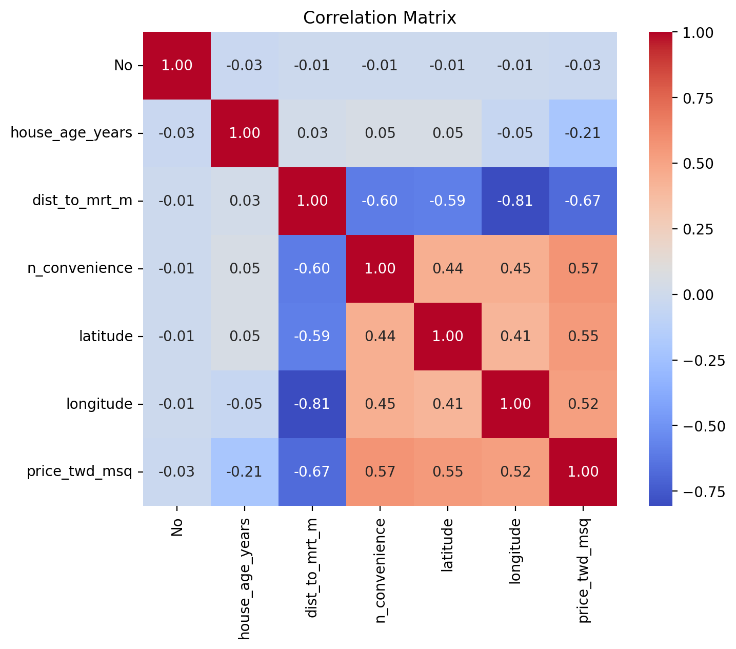

Draw a scatter plot of n_convenience vs. price_twd_msq:

# Your code here

Draw a scatter plot of house_age_years vs. price_twd_msq:

# Your code here

Draw a scatter plot of distance to nearest MRT station vs. price_twd_msq:

sns.regplot(df_estate,x="dist_to_mrt_m", y="price_twd_msq");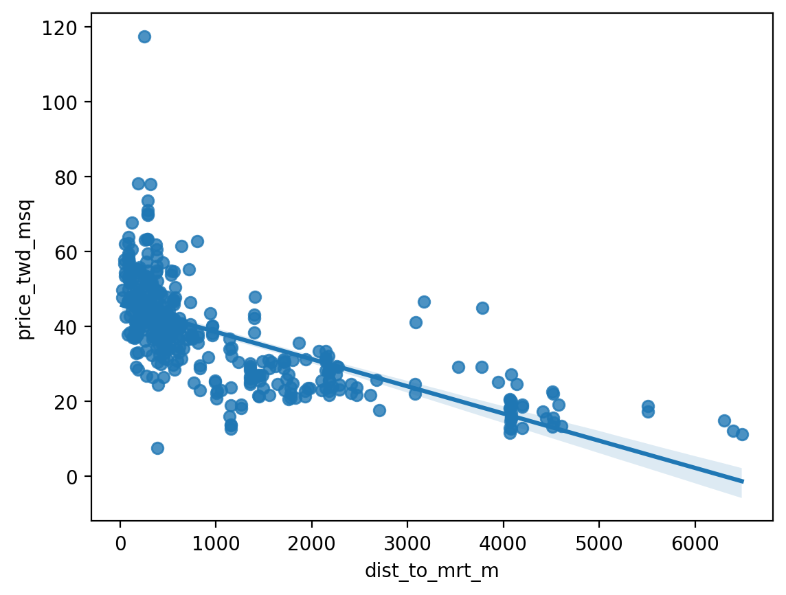

Plot a histogram of price_twd_msq with 10 bins, facet the plot so each house age group gets its own panel:

sns.histplot(df_estate, x="price_twd_msq", bins=10);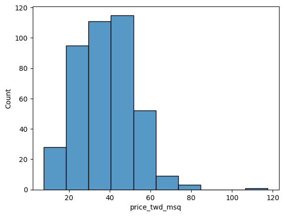

As we can see - the distribution of prices is not balanced/normal, so we need to normalize it with log:

df_estate['logprice'] = np.log(df_estate['price_twd_msq'])
df_estate['logdistance'] = np.log(df_estate['dist_to_mrt_m'])

Simple model¶

Run a linear regression of price_twd_msq vs. best, but only 1 predictor:

import statsmodels.api as sm

# Let's use 'dist_to_mrt_m' as the single best predictor
X = df_estate[['dist_to_mrt_m']]
y = df_estate['logprice']

# Add constant for intercept
X = sm.add_constant(X)

# Fit the model
model1 = sm.OLS(y, X).fit()

# Show the summary
print(model1.summary())

                            OLS Regression Results                            
==============================================================================
Dep. Variable:               logprice   R-squared:                       0.566
Model:                            OLS   Adj. R-squared:                  0.565
Method:                 Least Squares   F-statistic:                     537.3
Date:                Wed, 10 Jun 2026   Prob (F-statistic):           1.09e-76
Time:                        15:31:39   Log-Likelihood:                -26.939
No. Observations:                 414   AIC:                             57.88
Df Residuals:                     412   BIC:                             65.93
Df Model:                           1                                         
Covariance Type:            nonrobust                                         
=================================================================================
                    coef    std err          t      P>|t|      [0.025      0.975]
---------------------------------------------------------------------------------
const             3.8203      0.017    227.684      0.000       3.787       3.853
dist_to_mrt_m    -0.0002   1.01e-05    -23.180      0.000      -0.000      -0.000
==============================================================================
Omnibus:                       94.873   Durbin-Watson:                   2.119
Prob(Omnibus):                  0.000   Jarque-Bera (JB):              603.467
Skew:                          -0.799   Prob(JB):                    9.09e-132
Kurtosis:                       8.695   Cond. No.                     2.19e+03
==============================================================================

Notes:
[1] Standard Errors assume that the covariance matrix of the errors is correctly specified.
[2] The condition number is large, 2.19e+03. This might indicate that there are
strong multicollinearity or other numerical problems.

What do the above results mean? Write down the model and interpret it.

Discuss model accuracy.

Model diagnostics¶

4 Diagnostic plots¶

fig = plt.figure(figsize=(12, 10))
sm.graphics.plot_regress_exog(model1, 'dist_to_mrt_m', fig=fig)
plt.show()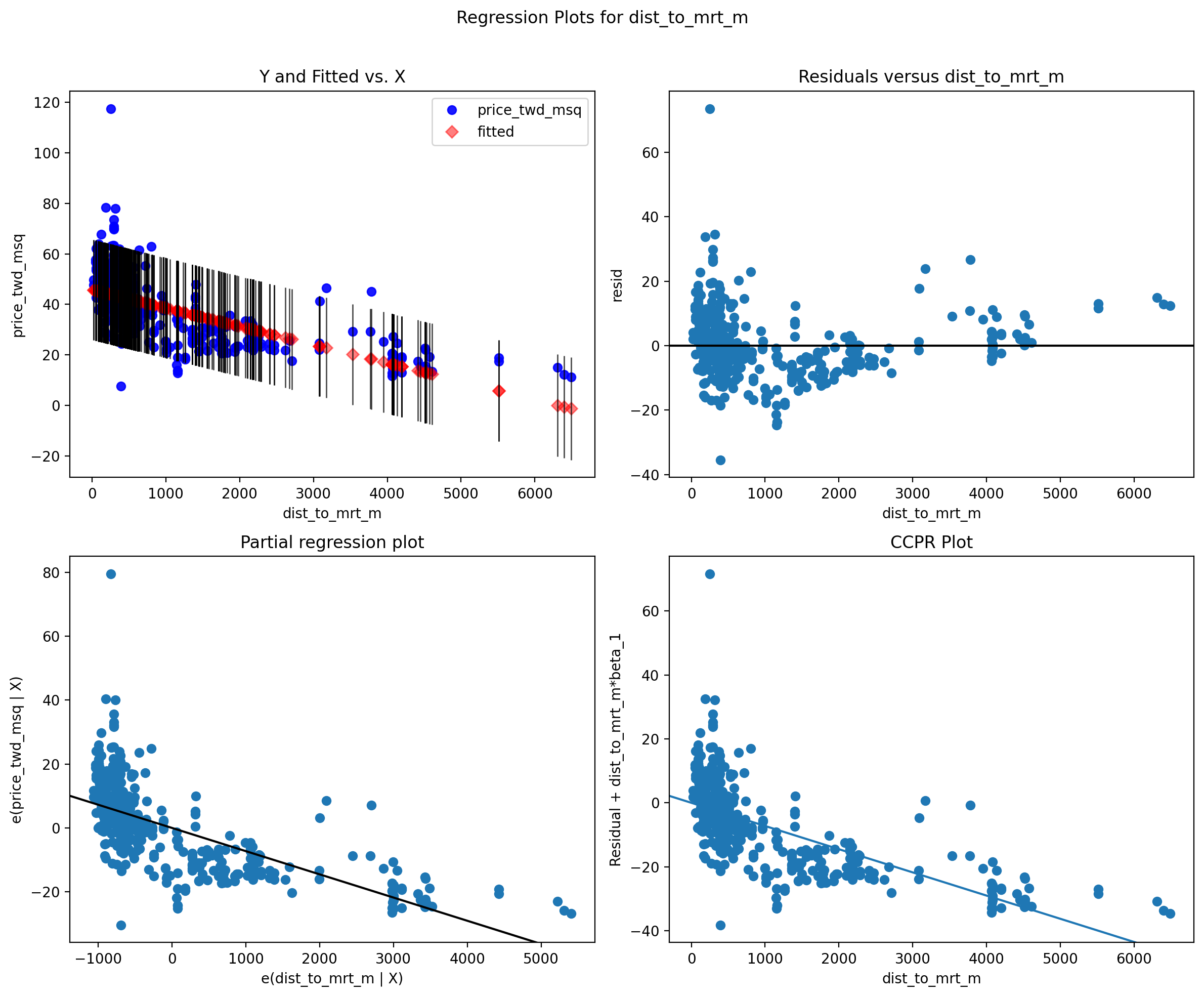

The four plots show...

Outliers and high levarage points:¶

fig, ax = plt.subplots(figsize=(8, 6))
sm.graphics.influence_plot(model1, ax=ax, criterion="cooks")
plt.title("Influence Plot (Outliers and High Leverage Points)")
plt.show()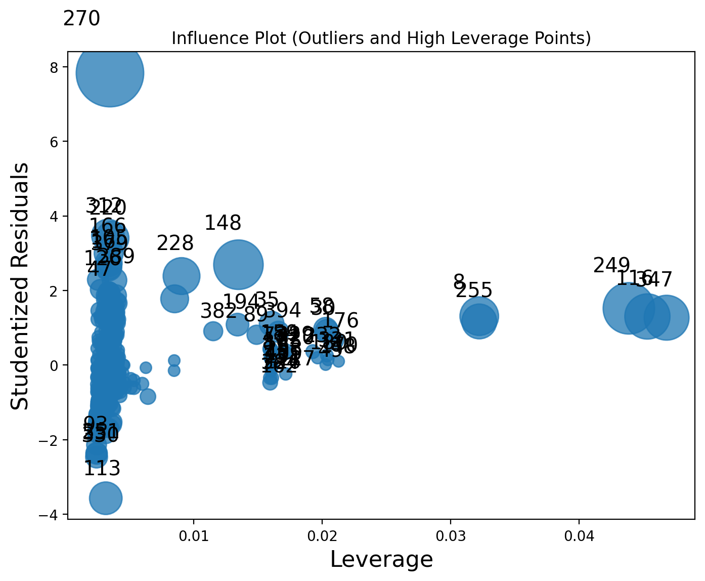

Discussion:

Multiple Regression Model¶

Test and training set¶

We begin by splitting the dataset into two parts, training set and testing set. In this example we will randomly take 75% row in this dataset and put it into the training set, and other 25% row in the testing set:

# One-hot encoding for house_age_cat_str in df_estate using get_dummies
house_age_dummies = pd.get_dummies(df_estate['house_age_cat_str'], dtype=int)
house_age_dummies = house_age_dummies.rename(columns={
  '0-15': 'house_age_0_15',
  '15-30': 'house_age_15_30',
  '30-45': 'house_age_30_45'
})

df_estate = pd.concat([df_estate, house_age_dummies], axis=1)
df_estate.head()

from sklearn.model_selection import train_test_split

# 75% training, 25% testing, random_state=12 for reproducibility
train, test = train_test_split(df_estate, train_size=0.75, random_state=12)

Now we have our training set and testing set.

Variable selection methods¶

Generally, selecting variables for linear regression is a debatable topic.

There are many methods for variable selecting, namely, forward stepwise selection, backward stepwise selection, etc, some are valid, some are heavily criticized.

I recommend this document: https://www.stat.cmu.edu/~cshalizi/mreg/15/lectures/26/lecture-26.pdf and Gung’s comment: https://stats.stackexchange.com/questions/20836/algorithms-for-automatic-model-selection/20856#20856 if you want to learn more about variable selection process.

[If our goal is prediction]{.ul}, it is safer to include all predictors in our model, removing variables without knowing the science behind it usually does more harm than good!!!

We begin to create our multiple linear regression model:

import statsmodels.formula.api as smf
model2 = smf.ols('logprice ~ dist_to_mrt_m + house_age_0_15 + house_age_30_45', data = df_estate)
result2 = model2.fit()
result2.summary()

What about distance to mrt? Please plot its scatterplot with the dependent variable and verify, if any transformation is needed:

# Your code here

# If any transformation is necessary, please estimate the Model3 with the transformed distance to mrt.

Discuss the results...

Error measures (formulas)¶

Mean Squared Error (MSE) - average squared residual; measures typical squared deviation of predictions from true values:

\mathrm{MSE}=\frac{1}{n}\sum_{i=1}^{n}(y_i-\hat{y}_i)^2

(1)

Residual Mean Squared Error (MSE_resid) - sum of squared residuals divided by residual degrees of freedom (p = number of parameters including intercept):

\mathrm{MSE}_{resid}=\frac{\sum_{i=1}^{n}(y_i-\hat{y}_i)^2}{n-p}

(2)

Residual Standard Error (RSE) - square root of MSE_resid; gives typical residual size in the original units of y:

\mathrm{RSE}=\sqrt{\mathrm{MSE}_{resid}}

(3)

Root Mean Squared Error (RMSE) - often computed on a test/validation set of size m; interpretable in y units:

\mathrm{RMSE}=\sqrt{\frac{1}{m}\sum_{i=1}^{m}(y_i-\hat{y}_i)^2}

(4)

Mean Squared Prediction Error (MSPE) - MSE computed on held-out data — measures out-of-sample prediction accuracy:

\mathrm{MSPE}=\frac{1}{m}\sum_{i=1}^{m}(y_i-\hat{y}_i)^2

(5)

Notes:

Use RSE (or mse_resid) to assess in-sample residual variability adjusted for model degrees of freedom.
Use RMSE/MSPE to evaluate prediction error on test or validation sets.
Compare values only across models with the same response scale.

#Calculating residual standard error of Model1
mse_result1 = model1.mse_resid
rse_result1 = np.sqrt(mse_result1)
print('The residual standard error for the MODEL 1 is:',np.round(mse_result1,3))

The residual standard error for the MODEL 1 is: 0.067

#Calculating residual standard error of Model2
mse_result2 = result2.mse_resid
rse_result2 = np.sqrt(mse_result2)
print('The residual standard error for the MODEL 2 is:',np.round(rse_result2,3))

---------------------------------------------------------------------------
NameError                                 Traceback (most recent call last)
Cell In[12], line 2
      1 #Calculating residual standard error of Model2
----> 2 mse_result2 = result2.mse_resid
      3 rse_result2 = np.sqrt(mse_result2)
      4 print('The residual standard error for the MODEL 2 is:',np.round(rse_result2,3))

NameError: name 'result2' is not defined

Looking at model summary, we see that variables .... are insignificant, so let’s estimate the model without those variables:

# Estimate next model here

Evaluating multi-collinearity¶

There are many standards researchers apply for deciding whether a VIF is too large. In some domains, a VIF over 2 is worthy of suspicion. Others set the bar higher, at 5 or 10. Others still will say you shouldn’t pay attention to these at all. Ultimately, the main thing to consider is that small effects are more likely to be “drowned out” by higher VIFs, but this may just be a natural, unavoidable fact with your model.

Variance Inflation Factor (VIF)¶

VIF formula for predictor j:

\mathrm{VIF}_j = \frac{1}{1 - R_j^2}

(6)

Where $R_j^2$ is the coefficient of determination obtained from regressing predictor $X_j$ on the remaining predictors (i.e. regression $X_j \sim$ other $X$ ).

Interpretation:

VIF measures how much the variance of a regression coefficient is inflated due to multicollinearity with other predictors.
Higher VIF indicates stronger collinearity; common thresholds are VIF > 5 (worth investigating) and VIF > 10 (serious problem).

A related measure is tolerance: $\mathrm{tolerance}_j = 1 - R_j^2 = \frac{1}{\mathrm{VIF}_j}$ .

Practical steps:

Compute VIF for all predictors.
If some VIFs are high, consider removing or combining correlated variables, applying regularization (e.g., Ridge), or transforming variables.

from statsmodels.stats.outliers_influence import variance_inflation_factor
X_vif = df_estate[['dist_to_mrt_m', 'house_age_0_15', 'house_age_30_45']].copy()
X_vif = X_vif.fillna(0)  # Fill missing values if any

# Add constant (intercept)
X_vif = sm.add_constant(X_vif)

# Calculate VIF for each feature
vif_data = pd.DataFrame()
vif_data["feature"] = X_vif.columns
vif_data["VIF"] = [variance_inflation_factor(X_vif.values, i) for i in range(X_vif.shape[1])]

print(vif_data)

           feature       VIF
0            const  4.772153
1    dist_to_mrt_m  1.061497
2   house_age_0_15  1.399276
3  house_age_30_45  1.400308

Discuss the results...

Finally we test our best model on test dataset (change, if any transformation on dist_to_mrt_m was needed):

# Prepare test predictors (must match training predictors)
X_test = test[['dist_to_mrt_m', 'house_age_0_15', 'house_age_30_45']].copy()
X_test = X_test.fillna(0)
X_test = sm.add_constant(X_test)

# True values
y_test = test['price_twd_msq']

# Predict using model2
y_pred = result2.predict(X_test)

# Calculate RMSE as an example metric
from sklearn.metrics import mean_squared_error
rmse = np.sqrt(mean_squared_error(y_test, y_pred))
print(f"Test RMSE: {rmse:.2f}")

Test RMSE: 8.38

Interpret results...

Variable selection using best subset regression¶

Best subset and stepwise (forward, backward, both) techniques of variable selection can be used to come up with the best linear regression model for the dependent variable price_twd_msq:

# Best subset selection using sklearn's SequentialFeatureSelector (forward and backward)
from sklearn.feature_selection import SequentialFeatureSelector
from sklearn.linear_model import LinearRegression

# Prepare predictors and target
X = df_estate[['dist_to_mrt_m', 'n_convenience', 'house_age_0_15', 'house_age_15_30', 'house_age_30_45']]
y = df_estate['logprice']

# Initialize linear regression model
lr = LinearRegression()

# Forward stepwise selection
sfs_forward = SequentialFeatureSelector(lr, n_features_to_select='auto', direction='forward', cv=5)
sfs_forward.fit(X, y)
print("Forward selection support:", sfs_forward.get_support())
print("Selected features (forward):", X.columns[sfs_forward.get_support()].tolist())

# Backward stepwise selection
sfs_backward = SequentialFeatureSelector(lr, n_features_to_select='auto', direction='backward', cv=5)
sfs_backward.fit(X, y)
print("Backward selection support:", sfs_backward.get_support())
print("Selected features (backward):", X.columns[sfs_backward.get_support()].tolist())

Forward selection support: [ True  True False False False]
Selected features (forward): ['dist_to_mrt_m', 'n_convenience']
Backward selection support: [ True  True False False  True]
Selected features (backward): ['dist_to_mrt_m', 'n_convenience', 'house_age_30_45']

Comparing competing models¶

import statsmodels.api as sm

# Example: Compare AIC for models selected by forward and backward stepwise selection

# Forward selection model
features_forward = X.columns[sfs_forward.get_support()].tolist()
X_forward = df_estate[features_forward]
X_forward = sm.add_constant(X_forward)
model_forward = sm.OLS(y, X_forward).fit()
print("AIC (forward selection):", model_forward.aic)

# Backward selection model
features_backward = X.columns[sfs_backward.get_support()].tolist()
X_backward = df_estate[features_backward]
X_backward = sm.add_constant(X_backward)
model_backward = sm.OLS(y, X_backward).fit()
print("AIC (backward selection):", model_backward.aic)

# You can print summary for the best model (e.g., forward)
print(model_backward.summary())

AIC (forward selection): 26.880219773672252
AIC (backward selection): 15.525426215434436
                            OLS Regression Results                            
==============================================================================
Dep. Variable:               logprice   R-squared:                       0.612
Model:                            OLS   Adj. R-squared:                  0.609
Method:                 Least Squares   F-statistic:                     215.5
Date:                Wed, 10 Jun 2026   Prob (F-statistic):           6.58e-84
Time:                        15:50:12   Log-Likelihood:                -3.7627
No. Observations:                 414   AIC:                             15.53
Df Residuals:                     410   BIC:                             31.63
Df Model:                           3                                         
Covariance Type:            nonrobust                                         
===================================================================================
                      coef    std err          t      P>|t|      [0.025      0.975]
-----------------------------------------------------------------------------------
const               3.6680      0.033    110.011      0.000       3.602       3.734
dist_to_mrt_m      -0.0002    1.2e-05    -16.078      0.000      -0.000      -0.000
n_convenience       0.0323      0.005      6.256      0.000       0.022       0.042
house_age_30_45    -0.1064      0.029     -3.666      0.000      -0.164      -0.049
==============================================================================
Omnibus:                       88.480   Durbin-Watson:                   2.090
Prob(Omnibus):                  0.000   Jarque-Bera (JB):             1010.007
Skew:                          -0.515   Prob(JB):                    4.78e-220
Kurtosis:                      10.582   Cond. No.                     4.76e+03
==============================================================================

Notes:
[1] Standard Errors assume that the covariance matrix of the errors is correctly specified.
[2] The condition number is large, 4.76e+03. This might indicate that there are
strong multicollinearity or other numerical problems.

From Best subset regression and stepwise selection (forward, backward, both), we see that the models selected by forward and backward selection may include different sets of predictors, depending on their contribution to model fit.

By comparing AIC values, the model with the lowest AIC is preferred, as it balances model complexity and goodness of fit.

In this case, the summary output for the best model (e.g., forward selection) shows which variables are most important for predicting price_twd_msq. This approach helps identify the most relevant predictors and avoid overfitting by excluding unnecessary variables.

Run model diagnostics for the BEST model:

fig = plt.figure(figsize=(12, 10))
sm.graphics.plot_regress_exog(model_backward, 'dist_to_mrt_m', fig=fig)
plt.show()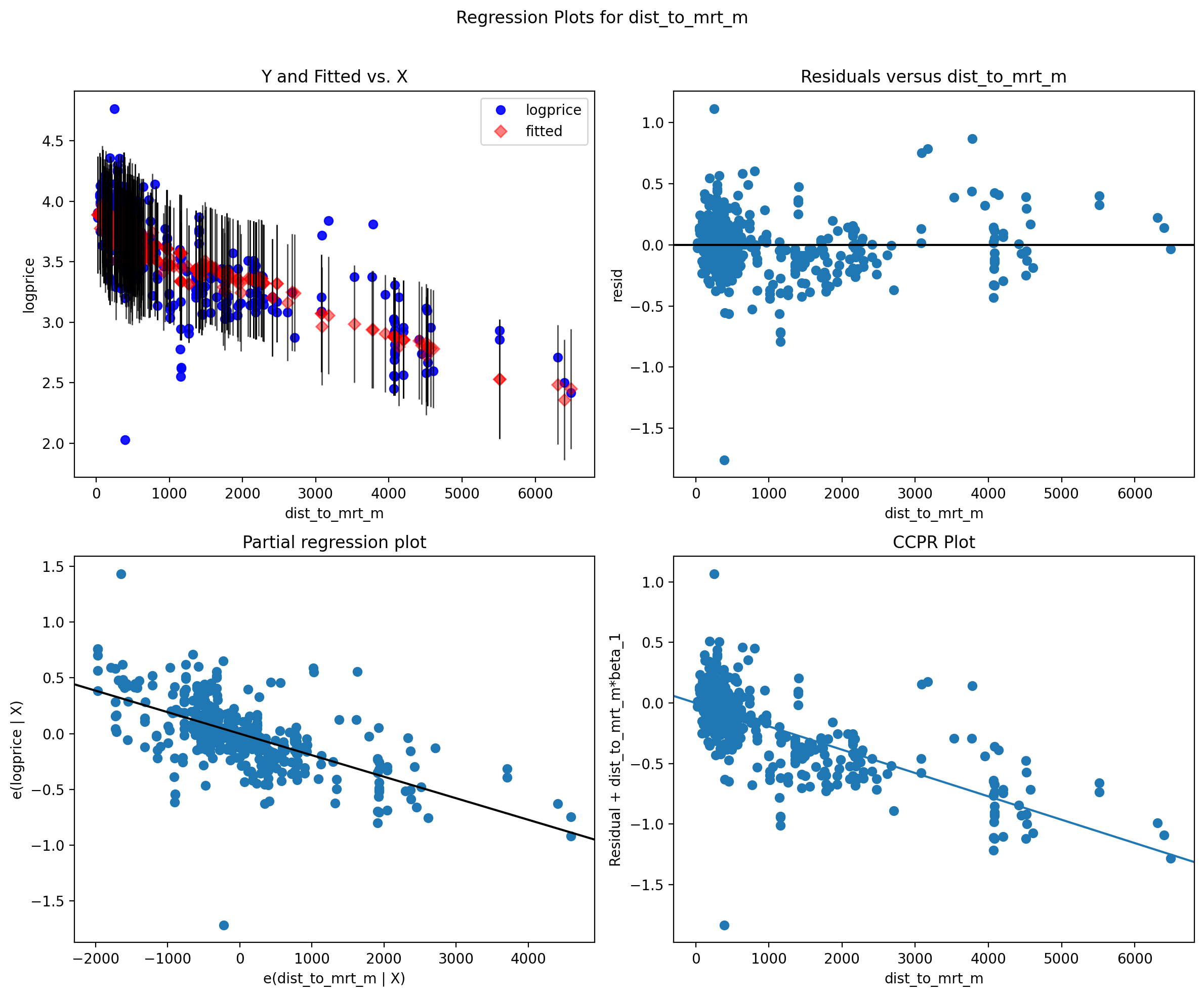

fig, ax = plt.subplots(figsize=(8, 6))
sm.graphics.influence_plot(model_backward, ax=ax, criterion="cooks")
plt.title("Influence Plot (Outliers and High Leverage Points)")
plt.show()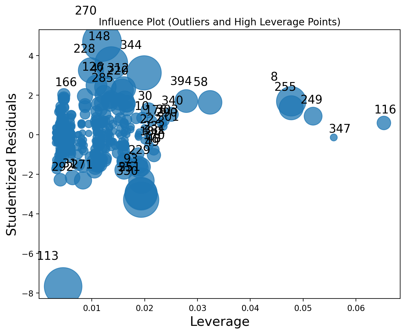

Finally, we can check the Out-of-sample Prediction or test error (MSPE):

X_test = test[features_forward].copy()
X_test = X_test.fillna(0)
X_test = sm.add_constant(X_test)

# True values
y_test = test['logprice']

# Predict using the best model (e.g., forward selection)
y_pred = model_forward.predict(X_test)

# Calculate MSPE (Mean Squared Prediction Error)
mspe = np.mean((y_test - y_pred) ** 2)
print(f"Test MSPE (out-of-sample): {mspe:.2f}")

Test MSPE (out-of-sample): 0.04

Cross Validation¶

In Python, for cross-validation of regression models is usually done with cross_val_score from sklearn.model_selection.

To get the raw cross-validation estimate of prediction error (e.g., mean squared error), use:

from sklearn.model_selection import cross_val_score
from sklearn.linear_model import LinearRegression

X = df_estate[['dist_to_mrt_m', 'house_age_0_15', 'house_age_30_45']]
y = df_estate['price_twd_msq']

model = LinearRegression()

# 5-fold cross-validation, scoring negative MSE (so we multiply by -1 to get positive MSE)
cv_scores = cross_val_score(model, X, y, cv=5, scoring='neg_mean_squared_error')

# Raw cross-validation estimate of prediction error (mean MSE)
cv_mse = -cv_scores.mean()
cv_rmse = np.sqrt(cv_mse)

print(f"Cross-validated MSE: {cv_mse:.2f}")
print(f"Cross-validated RMSE: {cv_rmse:.2f}")

Cross-validated MSE: 95.90
Cross-validated RMSE: 9.79

Summary¶

Do you understand all numerical measures printed in the SUMMARY of the regression report?
Why do we need a cross-validation?
What are the diagnostic plots telling us?
How to compare similar, but competing models?
What is VIF telling us?
How to choose best set of predictors for the model?